Solve your application with Machine Learning

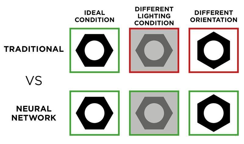
In the world of industrial automation, machine vision has long been the cornerstone of quality control. For decades, the gold standard has been the rule-based (or algorithmic) approach. Imagine you need to verify the presence of a hole on a metal bracket. Using a powerful vision software library, like the one integrated in OEVIS, an engineer designs a sequence of steps: acquire the image, apply a brightness threshold to create a binary image, run a blob analysis to find circular shapes, and measure their position and diameter. This method is deterministic, incredibly fast, and highly effective. It remains the best choice for metrology, alignment, counting, and any well-defined presence/absence task. The logic is explicit and can be described easily with a numeric rule, for example: "if the diameter is between 4.9mm and 5.1mm, the part is good."

But what happens when the rules become too complex to define?

Consider inspecting a product where defects are not about fixed measurements. Think of subtle scratches on a brushed metal surface, unpredictable texture flaws on a wooden part, or color variations in food products. How do you write a fixed rule for an unacceptable scratch? The number of conditions, exceptions, and lighting-dependent thresholds would become nearly impossible to manage.

This is where the Machine Learning (ML) paradigm offers a powerful and flexible alternative.

Instead of programming explicit rules, you teach the system by showing it examples. You provide the software with a curated dataset of images, carefully labeled as "Good" and "Bad." The Machine Learning model then analyzes this data and learns, on its own, the complex combination of features that best distinguish between the two classes. This shift from a "rule-based" to an "example-based" mindset is at the core of modern machine vision.

A complete machine vision software platform like OEVIS is designed to embrace this duality. It provides not only the robust, traditional tools for high-precision metrology but also a fully integrated suite of Machine Learning tools. This allows the two approaches to coexist and to work together to solve even more complex problems. To summarize the key differences between the two approaches, consider the following table.

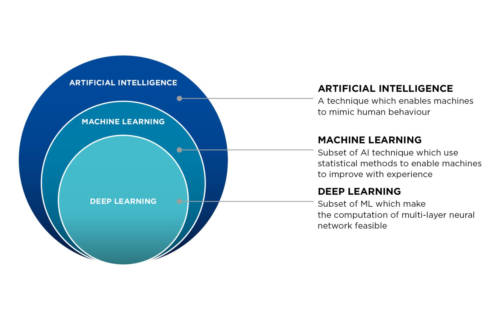
As you explore solutions for advanced machine vision applications, you will encounter two terms that are often used interchangeably: Machine Learning (ML) and Deep Learning (DL). While Deep Learning is technically a specialized subfield of Machine Learning, the distinction between the ML approach and the DL approach is a critical one for practical industrial applications. The primary difference is not in the goal, both aim to make accurate predictions from data, but in the method used to get there, specifically concerning feature extraction.

The Machine Learning Approach: Intelligence Guided by Expertise

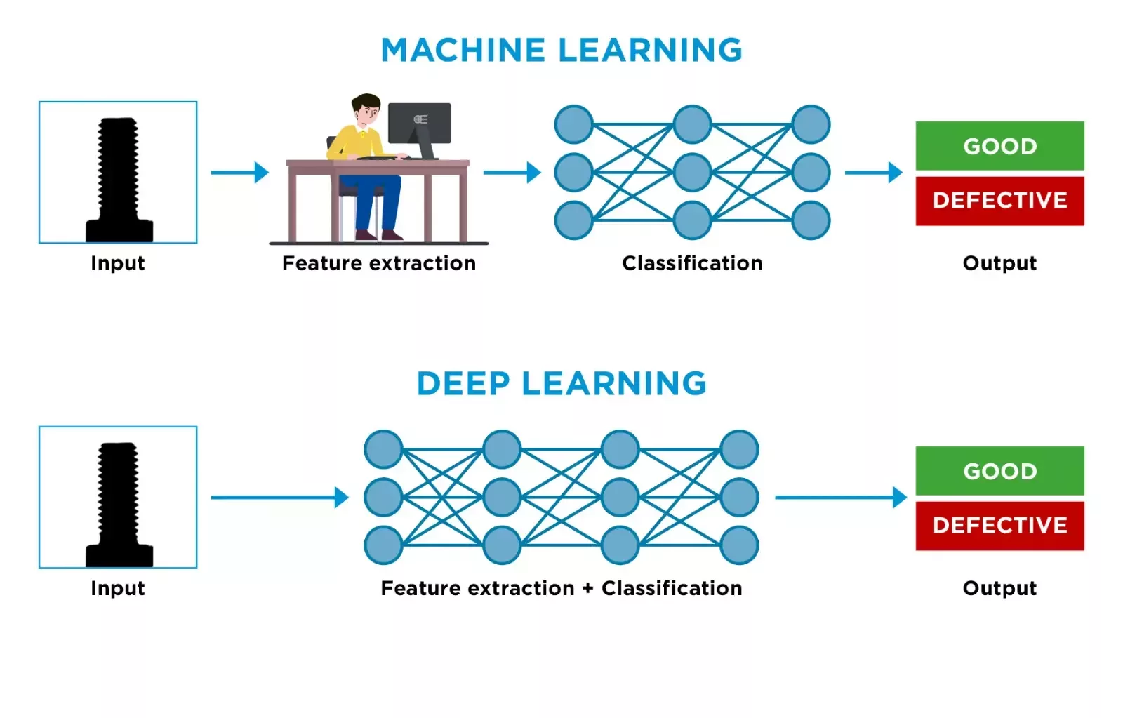
Machine Learning is best understood as a collaborative process where human expertise guides a powerful algorithm. The process doesn't start with raw pixels, but with the engineer's knowledge of what is important in the image. Imagine an experienced quality inspector. They don't just see a part; they subconsciously measure its key attributes such as the straightness of its edges, the uniformity of its surface, the roundness of its holes.

Machine Learning formalizes this process. The engineer uses a machine vision software like OEVIS to define and extract a set of precise, numerical parameters (features) from the image. This feature vector might include:

• Geometric Features: Area, perimeter, length, circularity, aspect ratio.
• Textural Features: Standard deviation of pixel intensity, entropy, contrast.
• Positional Features: X/Y coordinates, orientation.

This list of numbers effectively becomes a numerical summary, or a fingerprint, of the object in the image. This data is then fed to a classic ML model (like an SVM, KNN, or MLP). The model's job is to learn the complex patterns and relationships between these numbers to distinguish a "good" part from a "bad" one. The intelligence is therefore shared: the engineer uses their expertise to tell the system what to look at, and the algorithm learns how to judge what it sees.

The Deep Learning Approach: Intelligence Driven by Data

Deep Learning takes a fundamentally different approach. It is designed to be an "end-to-end" learning system that operates directly on raw data, using automatic feature extraction.

Instead of an engineer selecting features, a Deep Learning model, typically a Convolutional Neural Network (CNN), learns how to discover these features on its own. It does this through a hierarchical process that mimics a simplified model of human vision. The initial layers of the network learn to recognize very basic features like edges, corners, and color gradients. Subsequent layers combine these simple features into more complex concepts, like textures, patterns, or simple shapes. Deeper layers still can then combine these shapes to recognize object parts (like the thread of a screw or the handle of a cup) and, eventually, the entire object.

To achieve this, Deep Learning models are incredibly "data-hungry." Because the model starts with no prior knowledge, it must be trained on a massive dataset, often thousands, if not millions, of labeled images, to learn how to reliably distinguish features and ignore irrelevant variations. This process also demands heavy computational power, typically requiring high-end GPUs for many hours of training.

The Right Tool for the Machine Vision Application

The crucial takeaway is this: ML requires your expertise to extract the features; Deep Learning requires massive data and computational power to learn them automatically.

The table below provides a clear comparison for industrial automation and quality control contexts.

At the heart of every classic Machine Learning system lies a critical process that determines its success or failure: Feature Extraction. If the ML model is the brain that makes a decision, then feature extraction is the sensory system that perceives the world. It is the crucial step of translating a rich, visual scene into a clean, structured, and numerical format that a computer algorithm can understand.

Feature extraction is the process of measuring specific, relevant characteristics of an object in an image. The goal is to distill a complex picture down to a concise list of numbers, a feature vector, that serves as the object's unique numerical fingerprint. This process is what allows an ML model to work. The model does not see the image of a screw; it sees a feature vector like [Length: 45.2, Head Diameter: 8.1, Thread Count: 12, Straightness: 0.99], and it learns to associate this data with a class like "Good Screw."

How to Select the Right Features: A Practical Guide

Choosing the right features is a blend of scientific method and domain expertise. The goal is to find features that have high variance between classes but low variance within the same class. Here are some practical tips for selecting an effective feature set.

1. Start with your intuition. Before you even look at a feature list, ask yourself: "How would an expert human inspector tell these parts apart?" If they look for scratches, you need textural features. If they check for warping, you need geometric features that describe straightness or planarity. This initial brainstorming will guide you toward the right categories of features to explore.
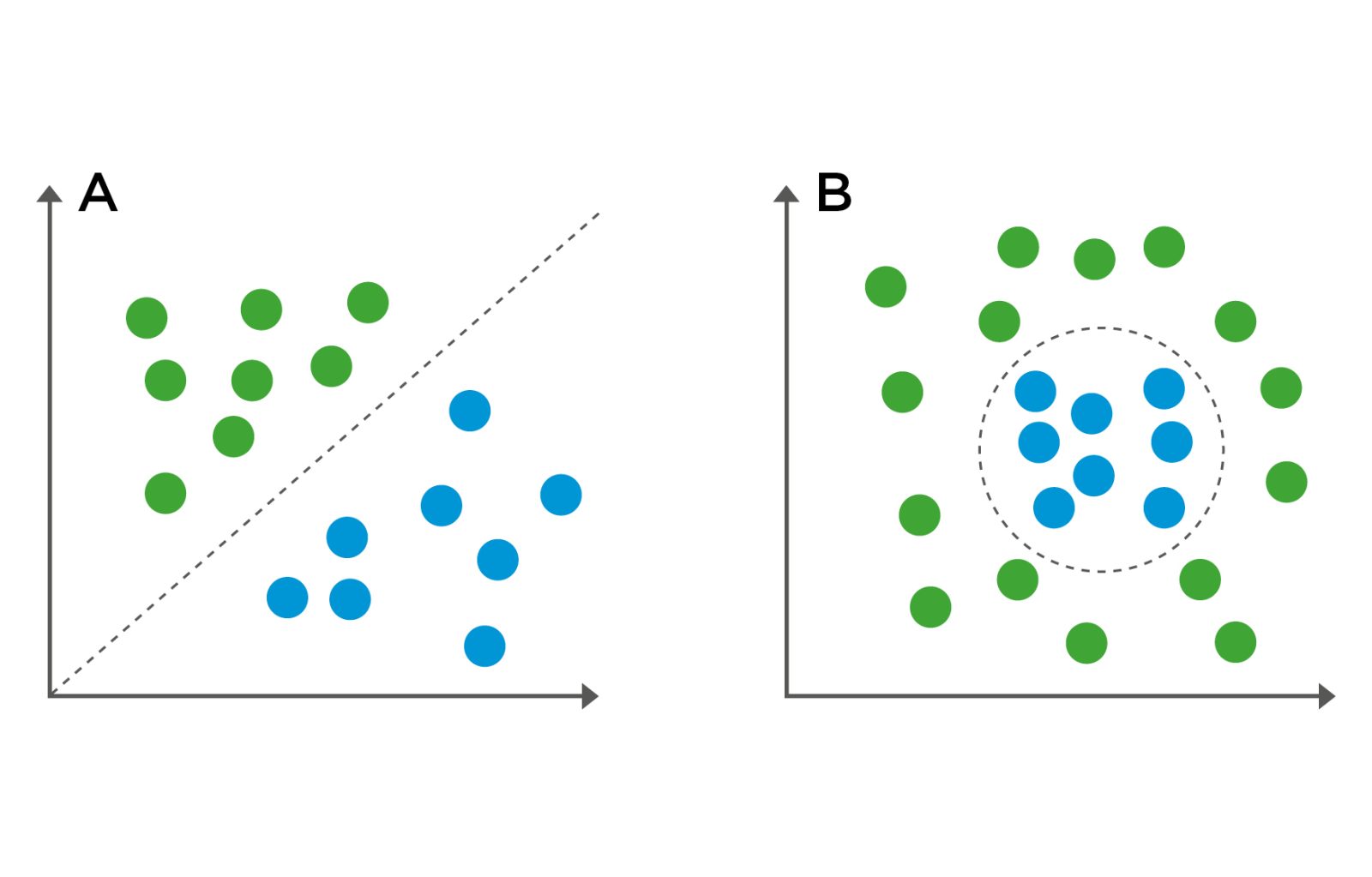
2. Visualize your features. This is the single most effective technique. Use a scatter plot to graph one feature against another for all your sample images. For example, plot "Area" on the X-axis and "Circularity" on the Y-axis. Color the points based on their class ("Good" vs. "Defective"). If you see distinct, well-separated clusters of colors, you have found powerful features. If the colors are all mixed together, those features are not effective at separating those classes.
3. Prioritize stability and relevance. A good feature must be relevant, meaning that its value must change significantly when the defect you're looking for appears. It also must be stable, so that its value must remain as constant as possible for good parts, even with slight variations in positioning or lighting. A feature that changes randomly is just noise.

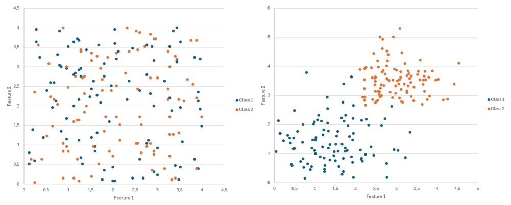
On the left an example of two features that are not useful for the classificatory, the graph representation shows that they are not distinctive. On the right an example of two distinctive feature, the graph representation clearly shows the two clusters.

How Many Features Should You Choose? The Curse of Dimensionality

It might seem intuitive to measure everything, but this is often counterproductive. Using too many features can harm the performance of your model, this is a concept known as the Curse of Dimensionality.

As you add more features (more dimensions), the space in which your data are represented becomes exponentially larger and sparser. This has two negative consequences:

• You need significantly more sample images to ensure you have enough data to define the class boundaries in this high-dimensional space.
• With too many features, the model might start learning from random noise and irrelevant correlations present in your specific training dataset. It becomes perfectly tuned to the training data but fails miserably when it sees new, real-world parts. This situation is known as Overfitting.

A good rule of thumb is to start with a small set of the most powerful features (2 to 5) and incrementally add more, validating at each step if the new feature improves classification accuracy on a separate test set. Often, a handful of well-chosen, stable features will outperform dozens of noisy, irrelevant ones.

The Critical Role of Image Acquisition

This brings us to a fundamental engineering truth: the quality and stability of your features are entirely dependent on the quality and stability of your images. This is the industrial application of the Garbage In, Garbage Out principle.

Consider the simple task of measuring the area of an O-ring from its shape.

• With a high-quality imaging system: Using a high-resolution camera, a telecentric lens, and a collimated backlight, you capture a perfectly sharp, high-contrast silhouette with no perspective distortion. The edge of the O-ring is defined with sub-pixel precision. The area feature, calculated by the vision software, will be highly stable and repeatable. A small cut in the O-ring will result in a small, but reliably detectable, change in the area.
• With a standard imaging system: Using a fixed focal length lens, the image may suffer from perspective error (the O-ring appears larger or smaller if it moves) and the edges can be blurry. If the backlight is uneven, the thresholding step becomes unreliable. The resulting area measurement will fluctuate randomly, even for the exact same part.

In the second scenario, the feature is noisy. A machine learning model trained on this data will be fundamentally unreliable. This is why investing in a high-performance optical setup is not a luxury; it is the foundational prerequisite for generating the clean, stable features that any successful Machine Learning system requires. Your hardware is the first and most critical part of your algorithm.

Once you have successfully engineered a stable and descriptive feature vector, the next step is to choose a classifier. The classifier is the ML model that will learn from your labeled feature data and ultimately make the final decision. Think of it as the judge that takes the numerical evidence (the feature vector) and delivers a verdict (the class label, e.g., "Pass" or "Fail"). In OEVIS there are three different classifiers available, in this section we are going to see how they work and when to choose them.

1. Support Vector Machine (SVM)

Imagine your feature data as points on a map, with good parts in one area and bad parts in another. The goal of an SVM is to find the single straightest, widest gap that separates these two groups. It doesn't just draw a line; it calculates the optimal boundary (called a hyperplane) that has the maximum possible margin from the nearest points of each class. These closest points, which support the boundary, are called support vectors. This focus on the boundary cases makes SVMs very robust.

The strengths of SVM are:

• High Accuracy: SVMs are renowned for their high accuracy and ability to generalize well to new data.
• Memory Efficient: Because the model is defined only by the critical support vectors, it can be very memory-efficient, even with large datasets.
• Effective in High-Dimensional Spaces: It performs well even when you have many features.

We suggest using SVM when:

• You have a clear-cut classification problem, especially binary (two-class) problems like Pass/Fail.
• The classes are linearly separable or can be made separable by a non-linear boundary.
• Interpretability is important. While not as clear as a simple threshold, the decision boundary is well-defined.

An example application is the verification of the correct assembly of a connector. The features might be the number of pins and area of the plastic housing. An SVM can create a very robust boundary to separate correctly assembled connectors from those with missing or bent pins.

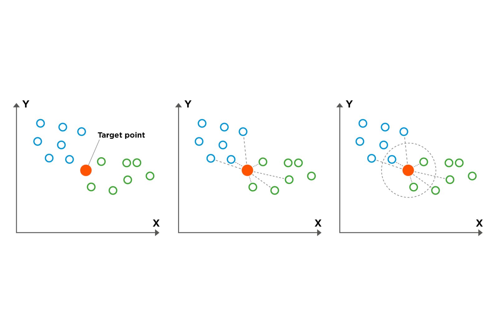
2. K-Nearest Neighbors (KNN)

KNN logic is: an object is likely to be similar to the objects near it. To classify a new, unknown part, the KNN algorithm looks at the K closest examples from the training data in the feature space. It then takes a majority vote: the new part is assigned the class that is most common among its K nearest neighbors.

The strengths of KNN are:

• Simplicity: The algorithm is very easy to understand and implement.
• Easy Training Phase: It doesn't build a model; it simply stores the entire training dataset. This makes it the best model for smaller datasets.
• Flexibility: It can naturally learn highly irregular and non-linear decision boundaries.

We suggest using KNN when:

• You have distinct clusters of classes in your feature space, but the boundaries between them are complex and not easily separated by a straight line.
• You want to get a baseline performance quickly due to its simple implementation.
• The classes are multi-modal, good parts might exist in two separate clusters in the feature space.

An application example is the sorting various types of fasteners (screws, bolts, rivets) that have come down a single conveyor. Based on features like length, head_diameter, and circularity, the parts form distinct clusters. KNN can easily classify a new part by seeing which cluster it falls into.

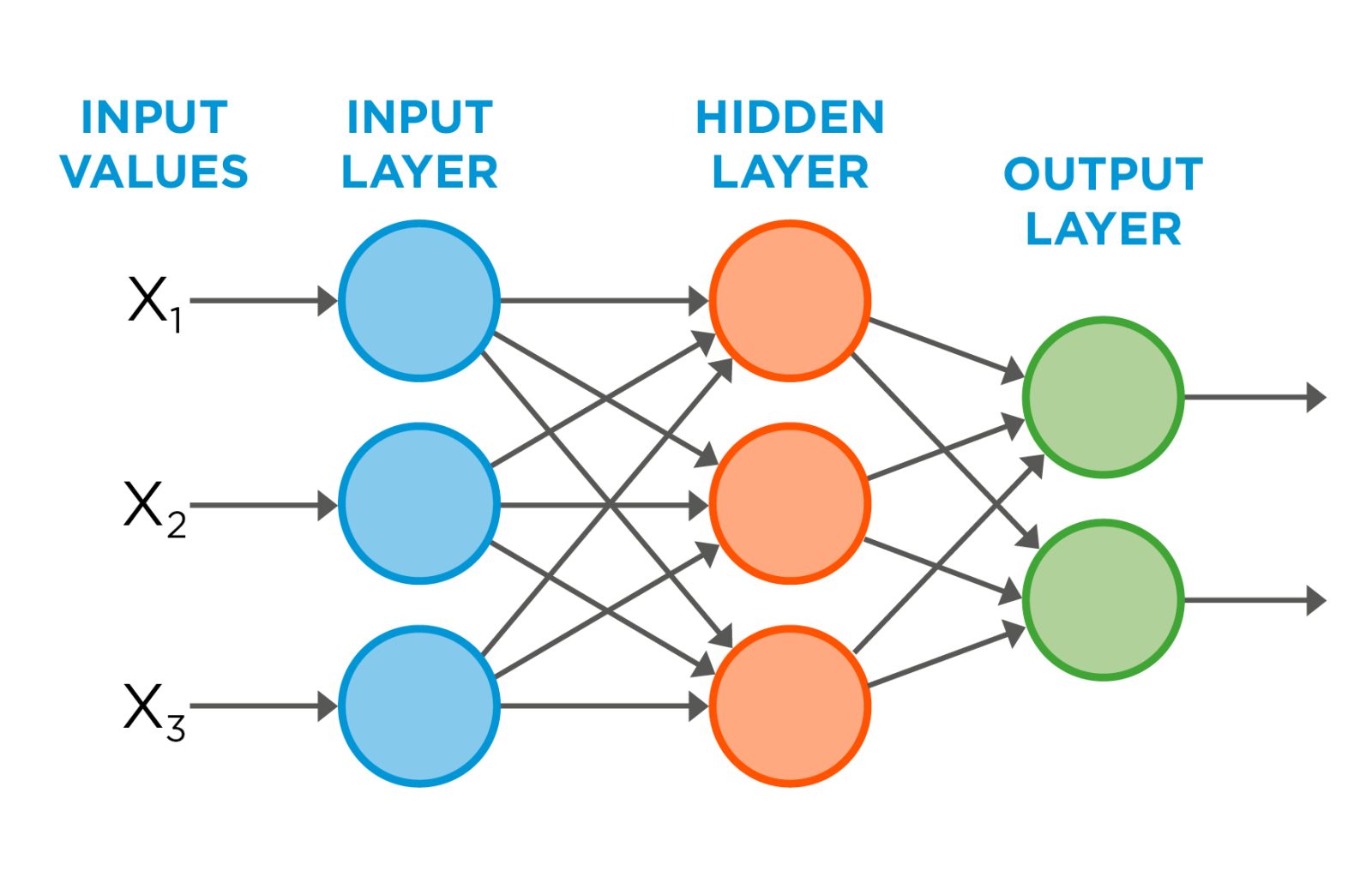
3. Multi-Layer Perceptron (MLP): The Flexible Learner

The MLP is the classic form of a neural network. It is composed of interconnected layers of neurons, starting with an input layer (where you feed your feature vector), one or more hidden layers, and an output layer (which provides the final classification). Each neuron applies a simple mathematical function to its inputs. By tuning the connections between neurons during training, the network can learn to approximate extremely complex, non-linear functions.

The strengths of MLP are:

• Maximum Flexibility: MLPs are universal approximators, meaning they can learn to model exceptionally complex and intricate relationships between features.
• Handles High Complexity: It is the go-to choice when the relationship between features and classes is not obvious or easily modeled by other classifiers.

We suggest using MLP when:

• You are facing a very challenging classification problem where SVM and KNN do not provide sufficient accuracy.
• You suspect there are complex, non-linear interactions between your features that determine the final class.
• You have a relatively large amount of training data to prevent the model from overfitting. Among the three models, MLP is the most data demanding.

A possible application is the inspection of high-end textiles for defects. The classification of a weave pattern as "Acceptable," "Slightly Frayed," or "Torn" might depend on a very subtle combination of a dozen textural and statistical features that must be extracted numerically and fed to the ML network. An MLP is best equipped to learn these subtle, high-dimensional patterns.

Developing a successful machine learning application is not a single action but a systematic process. Following a structured workflow is essential to ensure that the final system is accurate, robust, and maintainable. This chapter provides a repeatable, seven-step guide for taking your project from an idea to a fully deployed industrial solution.

Step 0: Feasibility Assessment for Machine Learning

Before committing to an ML deployment, confirm its necessity by evaluating the following critical factors against a rule-based solution:

Step 1: Define the Problem and Success Criteria

Before acquiring a single image, you must rigorously define your objective. A vaguely defined goal like finding defects is a recipe for failure.

• Define the Classes: What are the exact categories you need to differentiate? Be specific. Could be Good/Bad, or you can use precise classes like Acceptable, Scratch Defect, Stain Defect, and Deformation.

• Define the Business Goal: What is the desired business outcome? Examples include: "Reduce false rejects of acceptable parts by 80%" or “Automate the manual inspection of a part.”

• Define the Technical Success Metrics: How will you measure success? This should be a quantifiable target. For example: "The model must achieve an overall accuracy of 99.5% on the test dataset, with a cycle time (inference time) under 40 milliseconds per part."

Step 2: Design the Imaging System for Feature Stability

This is the most critical hardware step and the foundation of your entire project. As we established in Chapter 3, the goal is not just to get a clear image, but to acquire an image that makes the feature that you will use for the analysis as prominent and stable as possible.

Think backwards from your features. If you need to detect subtle scratches (a textural feature), your primary tool is lighting. A low-angle ring light or bar light will make the scratches stand out dramatically. If you need to classify parts based on precise dimensional measurements (geometric features), your primary tool is the lens. The choices you make here will directly impact the maximum possible performance of your ML model.

Step 3: Collect and Label the Dataset

This is often the most time-consuming phase, but it is indispensable. Your model will only be as good as the data it is trained on. Your dataset must capture the full range of real-world variability. This includes different production batches, acceptable variations in material color or finish, and examples of every single class you defined in Step 1.
One of the most common questions is: “how many images do I need for my dataset?”. The honest answer is: "it depends." The required dataset size is directly proportional to the complexity of your problem. However, we can provide some practical rules of thumb for classic Machine Learning applications. Please note that these numbers are based on experience and they do not represent a requirement.

• Simple problems: If you are classifying between 2-3 classes that are visually very distinct (e.g., separating screws from bolts), you can often start with a smaller dataset. A good starting point is 50 to 200 images per class.
• Moderately complex problems: If your classes have some visual overlap or a higher degree of in-class variation (e.g., classifying O-rings as "Good," "Slightly Deformed," "Broken"), you will need more examples for the model to learn the nuances. Aim for 200 to 500 images per class.
• Highly complex problems: If you are classifying defects that are very subtle, or parts with a great deal of natural variation (like wood or fabric), a larger dataset is necessary. Be prepared to collect 1,000 or more images per class.

Two principles are more important than these numbers alone. First, balance is key. Try to collect a roughly equal number of images for each class. A model trained on 500 "Good" images and only 20 "Bad" images will be heavily biased. This problem is known as class imbalance. Second, quality over quantity. A smaller, well-acquired dataset with consistent lighting and labeling is far more valuable than a huge dataset of noisy, inconsistent images.

While you acquire the dataset you have also to provide a label for your data. This process consists in assigning the ground truth class to every image. This process is of key importance in the development of your machine vision application since these will be the data on which the model will learn. It can happen that some samples could be classified differently by different people, it is important to agree on the classification of the images before proceeding further. Consistency here is key.

After you acquired your dataset, divide it into three different sets:

• Training set (70-80%): This is the data the ML model will learn from.
• Validation set (10-15%): This data is used to tune the model's parameters and to make decisions about which features to use. For KNN this is not used.
• Test set (10-15%): This data is kept completely separate and is used only once, at the very end, to provide an unbiased evaluation of the final model's performance.

Depending on the software, the split may need to be done manually. Split the dataset into two folders: train and test.

Step 4: Feature Extraction and Engineering

With your labeled dataset ready, it is time to translate the images into numerical feature vectors. Using the image processing tools in your vision software, you will develop a script or sequence to analyze each image and output the features you selected. This is an iterative process where you will extract, visualize, and refine your feature list. Please refer to the dedicated chapter for a more detailed guide on this.

Step 5: Train and Evaluate the Model

This is where the learning happens. You will need to select the best classifier for your application. This could be done by following the guide in the chapter dedicated to the classifier, but it can also be done empirically by trial and error. Once the classifier is selected, you need to train it by using the train and validation sets and then evaluate its performance based on the test set.

If at this stage, the results are not aligned with the expectations, you will need to look back at the whole process and try to find points where to improve. Usually, each classifier has some hyperparameters that can be tuned to change how the model learns so this is the first thing to investigate. Another point to deepen is the feature selection, try to understand if the features selected are the most representative for describing the problem. Finally, the training data could not be enough, or not well-balanced across the classes, so also this could be a point on which to improve.

Step 6: Deploy and Monitor

A trained model on a development PC is a lab experiment. A deployed model is a solution.

• Deployment (Inference): This involves loading your finalized model into your production inspection software (like OEVIS). The system will now perform real-time inference on live images.
• Monitoring: The job isn't over after deployment. Production conditions can drift. Plan for monitoring the model's ongoing performance and periodically retraining it with new data to ensure its accuracy remains high over the long term.

To demonstrate how the concepts and workflow discussed in this tech note come together, we will walk through a real-world application: the automated quality control of a metal surface.

The goal was to automate the inspection of a metal surface. The issue is with the finishing of the metal surface which must be finished correctly. Any scratch, missing material or differences of color is considered an error.

This example follows the seven-step process, showcasing how a combination of high-quality optics and intelligent software leads to a robust solution.

Step 0: Feasibility Assessment for Machine Learning

The ML approach is preferred for this application:

• Deterministic rules fail due to the inability to predict all possible defects, the high variability in features and lighting interactions, and the ambiguity between defects and the normal surface texture.
• Application constraints align with ML: A robust, large, and labeled dataset is available; the required output is classification; statistical error is acceptable; and the project timeline and maintenance demands are compatible with training and re-training.

Step 1: Define the problem and success criteria

There will be two output classes: OK and NOK, since we are not interested in classifying the single defect. The aim of the classificator should be to have an accuracy equal to or higher than 97%.

Step 2: Design the imaging system for feature stability

The surface of a metal part is highly reflective and has a strong texture which can be mistaken for a defect. This makes it a challenging imaging subject. The choice of hardware is not just important; it is the key to success. Our goal is to select an optical setup that makes all three defect types visible and measurable.

• Illumination: We made different tests using coaxial light, ring light and dome light. These tests showed that a flat Opto Engineering Ringlight provides the best illumination and contrast to see the defect. We used the LTRN023NW.
• Lens: To ensure that our images are consistent regardless of small variations in the part's placement and even small defects can be seen, a high-magnification Opto Engineering Telecentric Lens was selected. This eliminates perspective error, guaranteeing that a small scratch has the same apparent size in pixels, whether it's at the center or the edge of the field of view. We decided to use the TC4MHRP004-C.
• Camera: To obtain a good image we selected an ITA50-GM-10C. This camera allows enough resolution to clearly capture the defects.

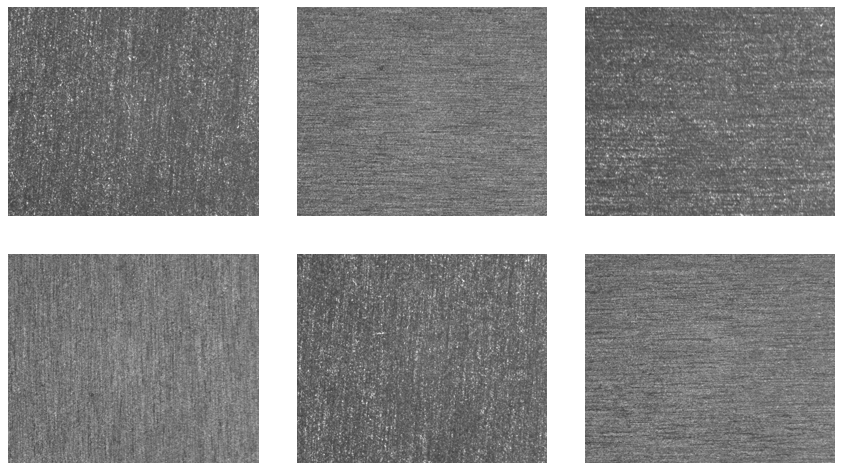
This hardware setup produces images where good surfaces are always similar, middle-gray, while defects manifest as clear deviations from this uniformity. Here you can find the images being captured divided into OK and NOK classes. The first group has the OK samples, while the second group has the NOK samples.

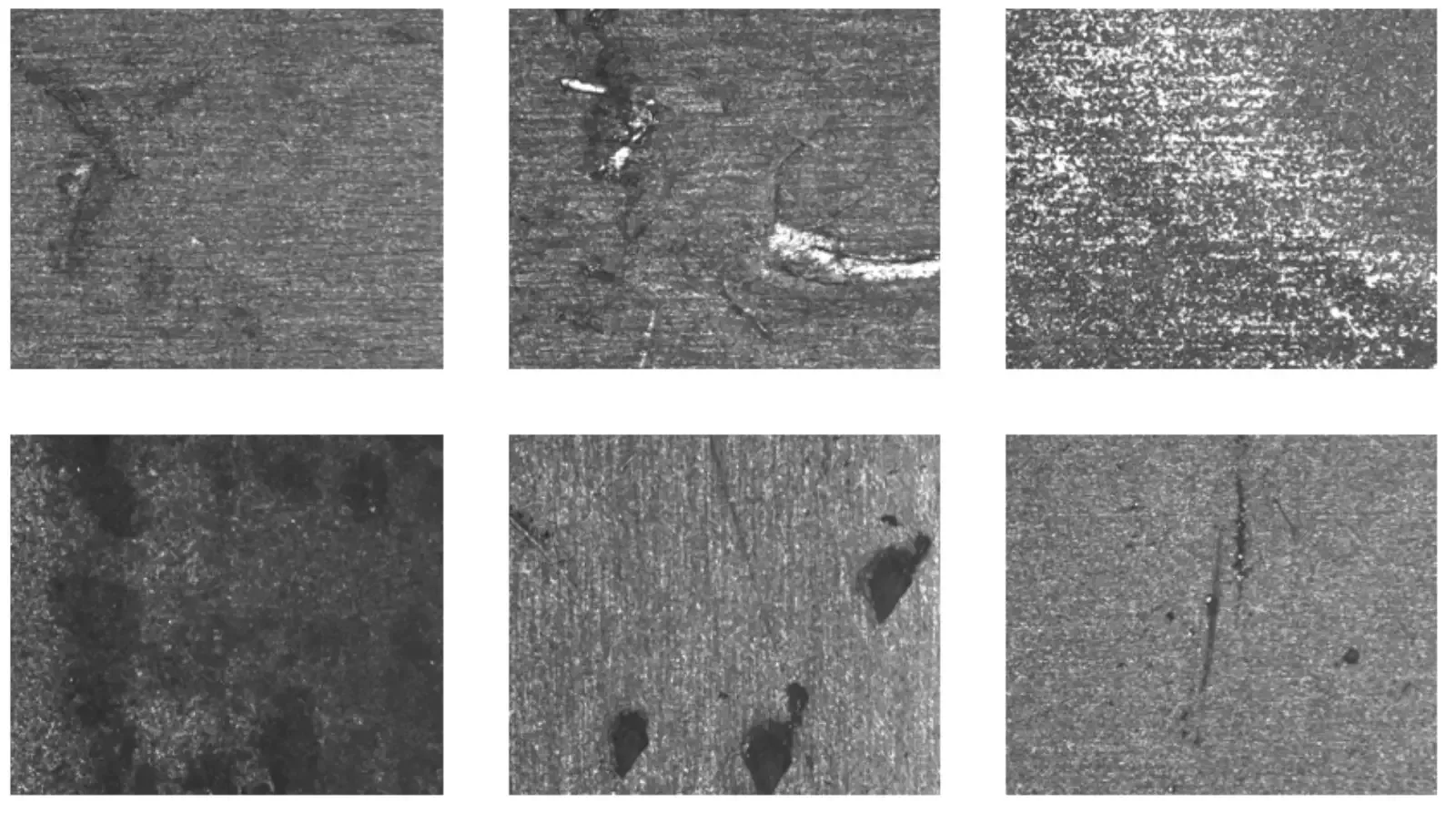
Step 3: Collecting and Labeling the Dataset

Following the guidelines from Chapter 5, we determined this to be a simple complex problem. We collected a balanced dataset to train our model.

• Dataset Size: A total of 100 images were captured.
  • 50 images of OK parts, ensuring we included samples from different production batches to capture the range of acceptable surface finish.
  • 50 images of NOK parts, with a mix of samples showing scratches, dents, and discoloration to ensure the model learns to recognize all defect types.

Dataset Split: The dataset was partitioned into Training (84 images) and Test (16 images) sets.

Step 4: Engineering the Features

With a high-quality image, the defects are now visually distinct. The next step is to quantify them using a feature vector. Since defects are essentially disruptions to the surface’s pattern, we chose four statistical and blob-based features, all easily calculated using OEVIS software.

1. Mean Gray Level: The average pixel brightness of the entire surface. This is very effective for detecting widespread discoloration. We choose this feature because we suppose that the presence of a defect will shift the average.
2. Variance of the Gray Level: A key textural feature. An OK part has a very low variance (all pixels are a similar shade of grey). A scratch or a sharp dent creates both dark and bright pixels, dramatically increasing the variance.
3. Number of Defect Blobs: Using a threshold to isolate pixels that are significantly darker than the mean, we can perform a blob analysis. This feature simply counts the number of resulting blobs.
4. Maximum Blob Area: This feature measures the area, in pixels, of the largest blob found. It helps to differentiate between a critical scratch and a tiny, irrelevant speck of dust.

For each image we will create a feature vector with all these values.

Step 5: Training and Evaluating the Model

• Classifier Choice: For this problem, we wanted to use a simple yet powerful model that works well when classes form distinct clusters in the feature space. The K-Nearest Neighbors (KNN) algorithm is a perfect candidate. Its intuitive logic ("a part is what its neighbors are") makes it easy to understand and validate. Also, this classifier works well when the number of data is low.
• Training: With KNN, the "training" phase is different from other models. As a "lazy learner," it doesn't build a complex internal model. Instead, it simply stores all 84 feature vectors from our training set. The real work happens during tuning, where we find the optimal value for 'K' (the number of neighbors to consider).
  • We tested several values for 'K'. With K=1, the model was too sensitive to single outliers.
  • With K=3 and K=5, the model became more stable, relying on a "majority vote" from a small group of neighbors.
  • By evaluating the accuracy on our 16 test images for each 'K', we determined that K=5 provided the best and most stable results, correctly classifying all validation images without being overly sensitive.

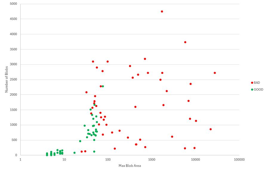
• Evaluation: Visualizing the features was very insightful. A plot of Maximum Blob Area vs Number of Blobs detected showed a clear separation: the OK parts formed a tight cluster at the origin (low variance, zero blobs), while the NOK parts were scattered further away with higher values for one or both features. This visual clustering confirmed that KNN was a suitable approach.
  

• Result: With the hyperparameter K set to 5, we performed a final evaluation on our 16 unseen test images. The model achieved 100% accuracy, correctly classifying all 16 parts. While this is a perfect score, it's important to note that a larger test set would be needed to have higher statistical confidence for a full-scale production deployment. However, for this application, it provided a strong validation of our approach.

Throughout this tech note, we have journeyed from the fundamental concepts of Machine Learning to a practical, step-by-step implementation of a real-world inspection system. We have seen how the "example-based" logic of ML can solve complex problems where traditional rule-based algorithms may struggle.

We have established a clear workflow:

• Assess if the use of Machine Learning is needed.
• Define your problem with precision.
• Design an imaging system to produce stable images.
• Collect and Label a representative dataset.
• Engineer a powerful feature vector to translate images into data.
• Train and Evaluate a classifier like SVM, KNN, or MLP.
• Deploy and Monitor the solution in a production environment.

By following this structured process, you can demystify Machine Learning and transform it from an abstract concept into a tangible, powerful tool for industrial automation.

If there is one single takeaway to remember from this guide, it is this: the success of your Machine Learning software is forged in the quality of your hardware and data. The most advanced classifier in the world is rendered useless if it is fed an unstable feature vector. And an unstable feature vector is the inevitable result of a noisy and inconsistent images.