ITALA® features
Connecting your camera to the lens
Dual exposure
Burst mode
Binning
Decimation
White balance
Color correction matrix
This chapter provides an overview of the ITALA® cameras main features, focusing on how to use each feature and explaining why it can improve your machine vision application overall performances.
We will insight into the technical details from the practical perspective of the user, providing suggestions and tips in order to get the best from our ITALA cameras and the overall vision systems.
Anyway, we recommend you to always refer to the camera manual and technical documentation if you are looking for further technical information about the implementation of a feature. Additionally, our technical support is always available for assisting you, just get in contact with us.
Let’s now start mastering ITALA® features and push the boundaries of your vision system up to a new level.
Connecting your camera to the lens
What it is
This working mode is related to the triggering strategy at the image sensor level. When the camera receives an input trigger in order to start a frame acquisition, at the image sensor level an electrical pulse starts the image sensor exposure time. Even at the sensor level, there is always a delay between the electrical pulse and the start of the sensor exposure. Such delay could change from one frame acquisition to another resulting in a time jitter on the delay between the trigger input and the image acquisition. By using the Fast Trigger Mode we avoid any time jitter between the trigger input and the starting of the image sensor exposure time.
Why it is interesting
In demanding high-speed applications the presence of a time jitter between the trigger input and the frame acquisition could affect the overall performance. Fast Trigger Mode image acquisition prevents any time jitter ensuring the most performant results.
The prevention of jitter time is useful when you want to guarantee good synchronization in your system. In particular, this feature helps in multi-camera systems in which you want to be sure of acquiring multiple images at the same time.
How to set fast trigger mode
To configure the fast trigger acquisition mode:
- Make sure the camera is idle, i.e.: not capturing images.
- Enable trigger acquisition mode by setting the TriggerMode parameter to ON.
- Set the SetTriggerOverlap parameter to OFF.

Technical considerations
- Fast Trigger Mode is only available when Trigger Overlap is disabled (i.e.: set to OFF).
- Fast Trigger acquisition mode is a design implementation that works at the image sensor level, its parameters are not accessible to the User.
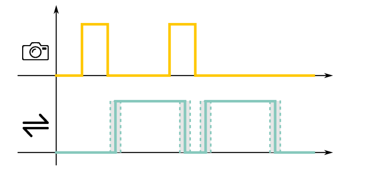
In the upper graph it is shown the behavior of the sensor exposure, while in the lower graph, the behavior of the sensor readout is depicted, over time on the horizontal axis.
When Trigger Overlap is set to Readout the latency between the exposure time and frame transfer is affected by a higher uncertainty. However, the following exposure can happen during the transfer of the previous frame between the sensor and the memory buffer.
With this mode it is possible to achieve a higher camera frame rate (limited by the communication interface) while having a lower frame transfer determinism.
Dual exposure
What it is
The Dual Exposure feature allows the acquisition of two frames in rapid succession by overlapping the first frame sensor readout period with the second frame sensor exposure period.
- When the first frame image sensor readout starts, the image sensor exposure of the second frame starts too.
- The image sensor exposure time of the second frame lasts as long as the image sensor readout of the first frame.
- Then the image sensor readout of the second frame must be finished before the next frame can be acquired.
Why it is interesting
Dual exposure is recommended for fast frame acquisitions on high speed lines where the sample features require different image exposure times or multiple lightings. It also could avoid using multi-camera systems.
This feature is useful when you need to acquire two images of a sample, for example with different light conditions. You can have a sample with a highly reflective part and a matte part, in this case you would want to make two exposures in order to have a useful amount of information on both parts of the sample.
Another interesting application of this would be with a CAGE optics, which is a system that integrates a backlight illumination and a ring light for a front light illumination. Using the Dual Exposure feature you can acquire two images in rapid succession with both the light setups.
How to set dual exposure
By default Dual Exposure is disabled, it is available only when trigger mode and trigger overlap are enabled and it must be used with a hardware trigger.To configure the Dual Exposure acquisition mode:
- Make sure the camera is idle, i.e., not capturing images.
- Enable trigger acquisition mode by setting the TriggerMode parameter to ON.
- Set the TriggerOverlap parameter to READOUT.
- Enable the dual exposure by setting the oeDualExposureEnable parameter to ON. Note: the AcquisitionBurstFrameCount parameter is then fixed to the value 2.
- Set the exposure time of the first frame (i.e.: EXPOSURE TIME 1 in the following picture) according to the standard ExposureMode parameter settings. Note: the exposure time duration can be set to either Timed or TriggerWidth.
Technical considerations
The following figure explains the Dual Exposure operation flow. The upper graph shows an incoming trigger signal over time, while the lower graph shows the exposure active over time.
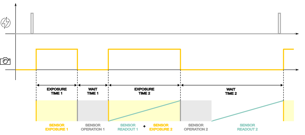
- After the input trigger is received the first frame exposure time starts. The EXPOSURE TIME 1 duration can be set by the user.
- After EXPOSURE TIME 1 is completed a WAIT TIME 1 is needed in order to complete sensor operations before the readout. This time represents the minimum time span between the two frames and it is fixed, refer to Itala user manual in order to retrieve WAIT TIME 1 duration.
- When the WAIT TIME 1 is finished the first frame readout and the second frame exposure time start. During this period the image sensor is performing two operations, the SENSOR READOUT 1 and the SENSOR EXPOSURE 2. Note that here the trigger overlap takes place.
- The EXPOSURE TIME 2 lasts as long as the SENSOR READOUT 1. This time is fixed, refer to Itala user manual in order to retrieve EXPOSURE TIME 2 duration.
- After EXPOSURE TIME 2 is completed a WAIT TIME 2 period is needed in order to:
- complete the SENSOR OPERATION 2
- complete the SENSOR READOUT 2
This time is fixed and no input triggers are accepted to start a new frame acquisition. Refer to Itala user manual in order to retrieve WAIT TIME 2 duration.
Burst mode
What it is
ITALA® cameras implement Burst Mode, taking advantage of its high-speed sensor, its onboard FPGA logic and onboard RAM memory by capturing and buffering frames at the sensor speed.
In burst mode acquisition, the camera acquires a selected number of frames at the sensor speed limit, while the FPGA manages the onboard frame buffer and transmission to the host. The frame transmission happens through the communication protocol of the camera interface. As a consequence, a “burst” of images can be acquired in quick succession at the image sensor speed limit.
Why it is interesting
Burst mode acquisition allows to work around the data transfer limitations of the camera interface (i.e.: Gig-E speed limit if 1G bit/s) and to acquire a burst of images at a higher frame rate, limited by the image sensor speed limit.
Burst mode can be useful when your objects come in batches at a rate that is higher than the communication interface frame rate. Using burst mode you can acquire the images of a single batch of samples at a rate higher than the communication interface transfer rate, the images will be stored in the buffer memory of the camera and then transferred to the PC at the camera interface speed before the next batch of samples needs to be acquired.
Another interesting application is when you need to acquire multiple images of a single object at a frequency higher than the communication interface frame rate. Using burst mode you can increase the acquisition frequency by saving the images in the camera buffer memory and then transferring them to the PC between two consecutive objects.
How to set Burst Mode
To configure the burst mode and set up burst image acquisition:
- Make sure the camera is idle, i.e., not capturing images.
- Enable frame burst triggering:
- Set the TriggerSelector parameter to FrameBurstStart.
- Set TriggerMode parameter to On.
- Set TriggerSource to the source that will generate the trigger.
- Set AcquisitionBurstFrameCount to a value higher than one.
Technical considerations
While the burst of frames is captured at the image sensor speed, the transmission of these frames to the host happens at the camera-to-host interface speed (e.g.: 1G bit/s in case of GigE interfaces).
The quantity of images that can be buffered is limited by the dimension of the image buffer, and in particular the dimension of the onboard RAM memory.
Such quantity also depends on the image dimension (i.e.: resolution, bit depth) and the acquisition speeds of the image sensor and the camera interface.
While the sensor pushes images in the buffer at a fast speed, the interface pops images out of the buffer at a slower speed.
As a consequence, burst mode acquisition always requires a waiting period between the acquisition of two consecutive “bursts of images” in order to prevent the onboard image buffer saturation.
Note that the maximum achievable image sensor speed is limited by both the exposure time and the image sensor readout time.
As general recommendations, we suggest to:
- set the AcquisitionFrameBurstCount at a value lower than the maximum quantity of images that can be stored in the onboard buffer. Such value can be calculated according to the following formula, which takes into consideration only the dimensions of the onboard RAM and of the acquired images.
- Be sure that the average input bandwidth is lower than the average output bandwidth.
- You can calculate the new Frame Rate using the number of frames in each burst and the number of bursts per second.
- The average output bandwidth is defined by the interface between the camera and the host (e.g.: 1G bit/s in the case of GigE interfaces).
Binning
What it is
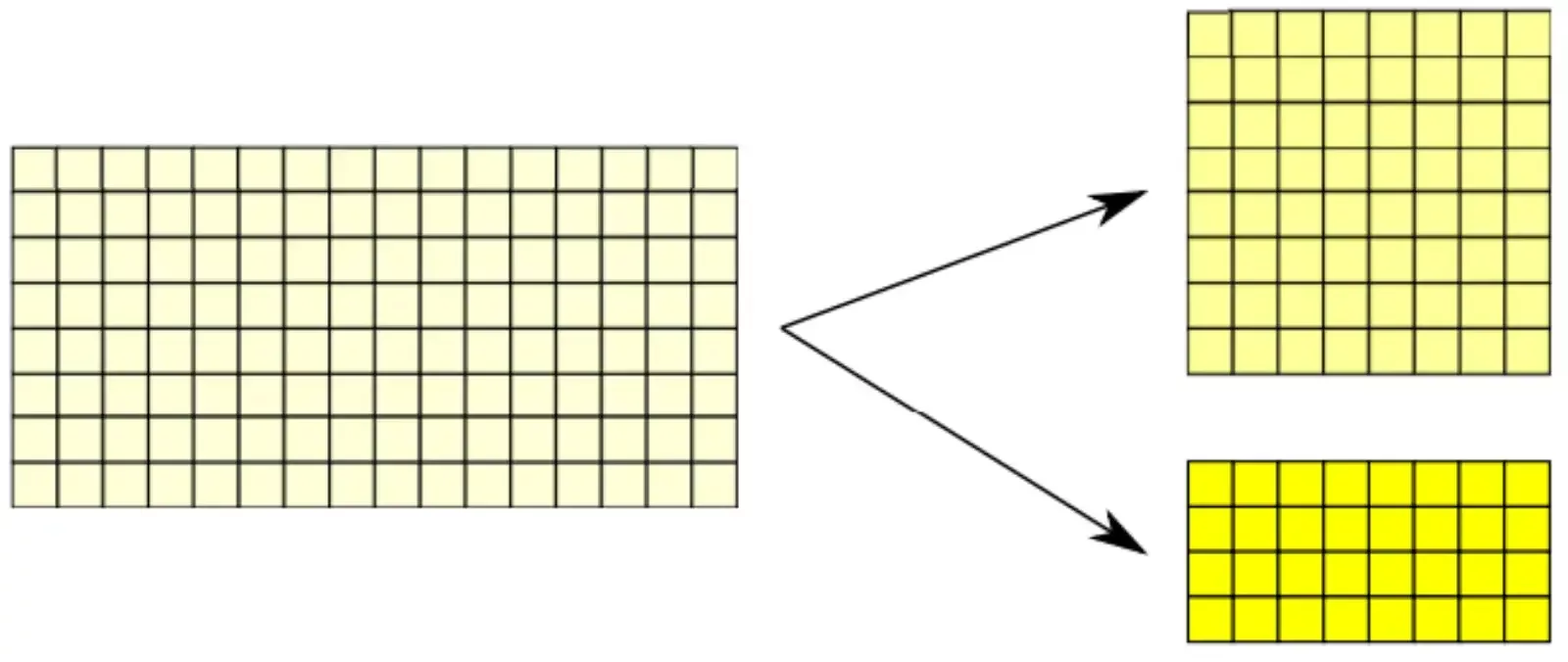
Binning allows the user to sum the gray level values of adjacent pixels into a single value, as if there is a single pixel that is the sum of them all.
The resulting image exhibits brighter intensity at the same image acquisition parameters (e.g.: same exposure time and gain) at the price of a loss in the effective image resolution.
Why it is interesting
Binning mode is useful to increase the camera sensitivity to light allowing setting a shorter exposure time at the same image brightness and eventually increasing the camera frame rate and reducing the pixel blur on moving objects.
In many machine vision applications the overall system resolution is limited by the optics while the camera resolution is often over-dimensioned with respect to the real application needs. In these cases reducing the camera resolution has a minor impact on the vision system capability to solve the overall application needs.
On the other hand, fast imaging is often a main constraint in machine vision because it results from compromises on the lighting, optics, camera and software sides.
Short exposure time is the limiting factor in particular on inline applications, where pixel blur is limiting the acquired image quality.
By increasing the light sensitivity binning mode also allows for either:
- set a shorter exposure time at the same lighting and optics conditions (e.g.: light intensity and optics aperture).
- get a brighter image at the same exposure time and gain, without modifications on lighting and optics.
- achieve a faster camera frame rate by reducing the exposure time at the same brightness on the resulting image acquired.
For example, in the case of a 2x2 binning we should expect the following:
- the vision system collects 4 times more light.
- the frame rate increases up to 4 times, also depending on the exposure time value and on the camera and the interface bandwidth (see following technical information).
- resolution decreases 4 times (2 horizontally and 2 vertically).
How to set Binning
By default, binning is disabled, in order to configure it:
- Connect the camera and make sure it is idle (i.e.: not capturing images).
- In the Image Format Control section set the BinningHorizontal, the value could be either 1, no binning, or 2, binning of a factor 2.
- In the same way, you can setBinningVertical value, either to 1 or 2.
Note that when binning is used, decimation is not available.
Technical considerations
The maximum allowed binning is 2x2.
In case a 2x1 binning is performed the image resolution along the horizontal axis will become half while the resolution along the vertical axis is preserved, while the overall image brightness is doubled (since two adjacent pixels have been combined).
In case a 2x2 binning is performed, the image resolution is a quarter of the initial one and both resolutions on the horizontal axis and vertical axis are halved, while the overall image brightness will be four times the initial one.
Note that different binning factors for horizontal and vertical axes, will make objects appear as distorted in the image.
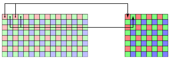
In case of color sensors, Bayer filter must be taken into account.
This is because with Bayer filter adjacent pixels have different chroma information. Therefore, binning is performed on alternate pixels. In this way the chroma information is not affected by any algorithm artifacts.
Binning is executed on the sensor only when a monochrome camera is used and a 2x2 binning is selected.
Moreover, not all second-generation Sony sensors have binning capabilities (this is sensor-specific). When binning is not executed on the sensor, it is performed by the onboard FPGA.
Some considerations are needed about the Depth of Field (DOF), since binning increases the pixel size, it could be thought that the DOF increases by the same factor. For example, if 2x2 binning is introduced then the pixel size becomes 2 times bigger on each side and, we could expect the DOF to increase 2 times accordingly. This is a wrong conclusion because the achievable DOF must take into account the application needs.
By definition, the DOF is “the maximum range where the object appears to be in acceptable focus”.
When binning is performed, the overall image resolution achievable by the vision system (which includes both the optics and the sensor resolutions) always decreases. Such resolution loss happens at both the WD and in the whole original DOF range.
On the other hand, thanks to the binning the image transitions are sharper, because these happen on less pixels. For example, if an image transition happens on 8 pixels without binning, it will happen on 4 pixels if a 2x2 binning is applied.
Despite the sharper transitions, the quantity of information in the image (i.e.: the image MTF) always decreases when the binning is performed, at both the WD and in the DOF range.
According to these considerations, the possibility to increase the DOF by performing the binning depends on the application. If the application does not require resolution but it requires sharp transitions (i.e.: some measurement applications), then binning could contribute to increasing the overall vision system DOF.
If the application requires high resolution, since binning does not allow to see more information in the acquired image, it generally should not be considered as a method in order to increase the overall vision system DOF.
In conclusion, the possibility to increase the DOF by introducing binning must be evaluated by testing the vision system performances according to the application requirements, and it can not be estimated by simply considering the pixel size increase.
Another common mistake is to consider the frame rate increase directly proportional to the binning factor. Taking again into consideration the previous example of a 2x2 binning, it could be thought that since the resolution is 4 times lower, the frame rate is 4 times higher. Also in this case the conclusion is wrong and further technical considerations are needed.
The camera frame rate is limited by both the exposure time and the camera readout time.
At the same image brightness, the binning could allow to decrease the exposure time proportionally to the binning factor.
Anyway, the exposure time is set by the user independently from the binning, and the possibility to decrease it when binning is introduced depends on the application needs.
How binning influences the camera readout time is more complex.
Binning is executed by the sensor only when a monochrome camera is used and when a 2x2 binning is selected.
Moreover, not all sensors have binning capabilities (this is sensor-specific).
When binning is not executed on the sensor, it is performed by the onboard FPGA.
When binning is performed by the sensor, it affects the overall readout speed of the camera both when it is limited by the readout speed of the sensor and when it is limited by the speed of the communication interface between the camera and the PC (i.e.: 1G bit/s in case of Gig-E).
When binning is executed by the onboard FPGA, it influences the camera readout time only if the readout bandwidth is limited by the bandwidth of the communication interface.
If the camera readout speed is limited by the sensor readout speed, for example because a small sensor's ROI has been selected, the introduction of a binning factor performed by the FPGA will not influece the resulting camera readout time.
When binning influences the camera's overall readout bandwith, the camera's readout speed is increased by a factor which is approximately proportional to the binning factor, because the amount of pixels to read is inversely proportional. However, at high speeds, some time-constant operations onboard the camera or the sensor may become non-negligible and may have an influence on the overall readout time of the camera.
In conclusion, while binning usually allows an increase in the camera frame rate, the actual increase in the frame rate must be considered on a case-by-case basis, because it depends on both the exposure time and the readout time of the camera, and may or may not be influenced by the binning factor set, considering the specifications of the sensor and the needs of the application. Often the best way to evaluate the actual increase in frame rate is to carry out a test.
Decimation
What it is
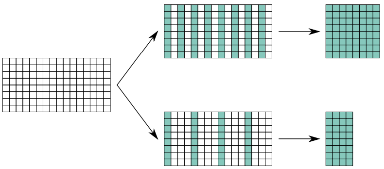
Decimation allows the user to discard pixels on the columns or rows of the sensor in order to increase the frame rate without any other changes in the camera parameters, at the price of a loss in the effective image resolution.
Why it is interesting
Decimation mode allows the user to increase the camera frame rate by reducing the amount of data output.In many machine vision applications the overall system resolution is limited by the optics while the camera resolution is often over-dimensioned with respect to the real application needs. In these cases reducing the camera resolution has a minor impact on the vision system capability to solve the overall application needs.
In these cases decimation is a very easy and convenient way to increase the camera frame rate. Since the image sensor dimensions are the same, no other modifications are required on other vision system components such as optics and lighting.
The possibility to set different decimation factors on the horizontal and vertical axis also allows the user a higher flexibility in setting the proper resolution, image ratio, and frame rate, tailoring the camera performances to the specific application needs.
How to set Decimation
By default decimation is disabled, in order to configure decimation:
- Connect the camera and make sure it is idle (i.e.: not capturing images).
- In the Image Format Control section set the Decimation Horizontal value. The allowed values are 1, 2 and 4.
- In the same way you can set the Decimation Vertical value.
Note that when decimation is used, binning is not available.
Technical considerations
Depending on the kind of decimation chosen, vertical, horizontal or both, the sensor will transmit data respectively every N rows or N columns, where N is the decimation factor.
For example:
- 2x1 decimation: only one pixel over two along the rows is considered, therefore the resulting image has half of the initial horizontal resolution, while vertical resolution is preserved.
- 4x1 decimation: only one pixel over four along the rows is acquired, as a consequence the horizontal resolution is reduced by a factor of 4, while vertical resolution is preserved.
The maximum allowed decimation is 4x4.
Note that different decimation factors for horizontal and vertical axes will make objects appear distorted in the image.
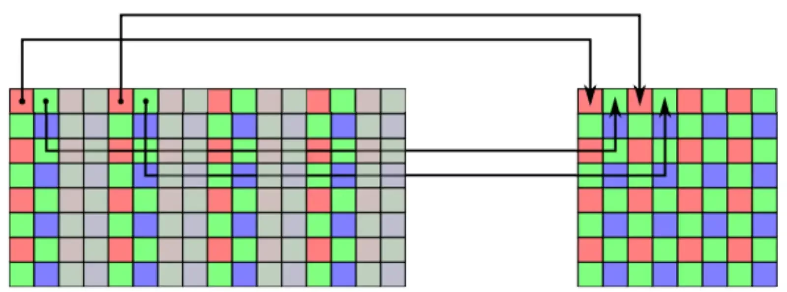
In case of color sensors, Bayer filters must be taken into account. Indeed, since adjacent pixels have different chroma information, decimation is performed by grouping pixels with alternate colors. In this way, chroma information is not affected by algorithm artifacts.
While decimation allows to increase the camera frame rate, it is important to note that the frame rate increase is not proportional to the decrease in resolution. Taking into consideration a 4x1 decimation, as well as a 1x4 or a 2x2, it could be thought that since the resolution is 4 times lower than the frame rate is 4 times higher. This conclusion is wrong and further considerations are needed.
The first reason is that the overall sensor operation time is the sum of the sensor exposure time and the sensor readout time.
Introducing the decimation decreases the quantity of pixels that should be output in during the sensor readout time, but it has no impact on the sensor exposure time.
In addition, the sensor readout time is not directly proportional to the quantity of pixels, because some time-constant operations are also needed on the sensor level.
It must also be considered that decimation on the vertical axis will increase frame rate more than decimation on the horizontal axis due to the design characteristics in the pixel readout at the sensor level.
Finally, the frame rate is still limited by the bandwidth of the connection interface to the host (i.e.: 1 Gb/s in case of GigE).
In conclusion, the actual frame rate increase should be considered on a case by case basis, it depends on the camera and the sensor part numbers, and it must be evaluated also by testing.
White balance
What it is
White balance is a feature that allows you to analyze and adjust the color channel information of each pixel in a captured image in order to compensate for any color casts caused by different lighting conditions and/or the difference in light sensitivity of the three color coordinates in a color sensor.
Why it is interesting
The “human visual system” achieves color constancy by perceiving white as white, regardless of different lighting conditions. When captured by digital cameras, images vary based on light temperature, making white objects appear reddish in warm light and bluish in cold light. White balance adjusts images to maintain visual consistency.
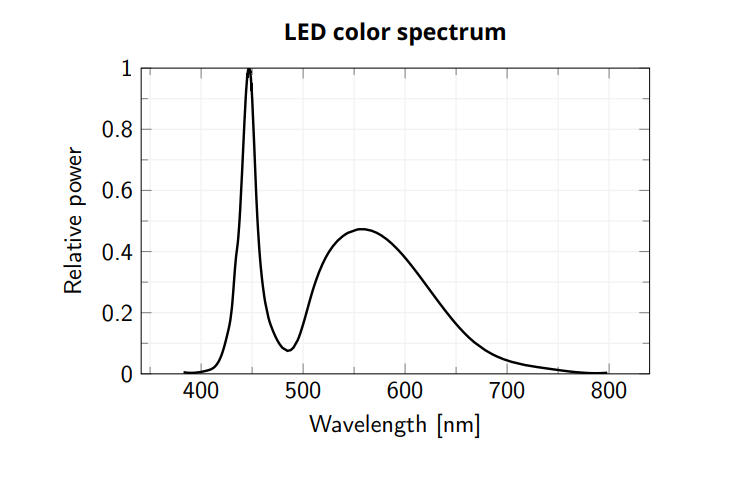
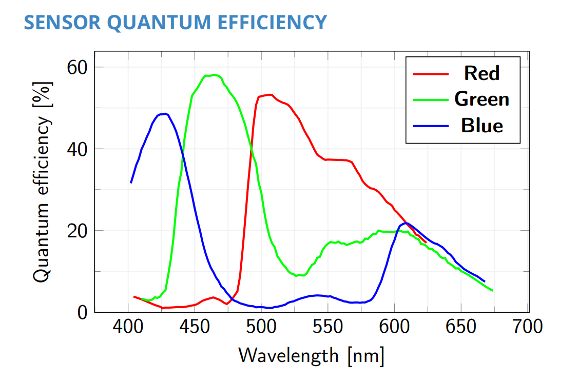
Digital camera sensors primarily measure light intensity, not wavelengths, necessitating RGB Bayer filters for color. These filters have variable spectral transmittance, while sensor sensitivity also varies among the light spectrum, and even from sensor to sensor among the same manufacturer.
The same variability should be expected in the application’s lighting conditions, which changes depending on the illuminator specifications, the sample characteristics and even from illuminator to illuminator among the same manufacturer and the same batch, or after some time of operation.
The use of white balance in a machine vision application ensures the consistent color representation of an image independent of any illumination variability or intrinsic differences in light sensitivity. This is particularly important for applications where color accuracy is crucial, such as color inspection, color sorting, or color analysis.
Machine vision softwares which take into consideration some types of color analysis must rely on an accurate color fidelity, which could have a great impact on the information extracted by the images and the application results.
How to set White Balance
By default white balance is enabled with some fixed values. The goal of this procedure is to find the best coefficient specific to your application. In order to configure white balance:
- Connect the camera and make sure that it is in free run acquisition.
- Make sure to insert a uniform-colored grey sample.
- Make sure that the sample covers all the Field of View (FOV). region of interest (ROI).
- Select the tab “Histogram” to see the histogram of the image, since it is not balanced you should see three curves centered at different values.
- You could draw a Region of Interest (ROI) to see the histogram of that area.
- Make sure that none of the three color channels are saturated, you can use the histogram tool to evaluate color saturation. In case of saturation, exposure must be adjusted before proceeding.
- Switch BalanceWhiteAuto either to “Once” or to “Continuous”.
- The histogram will change so that the three curves are centered around the same value, now the image is white balanced.
- If at the previous point you chose BalanceWhiteAuto to “Continuous”, now set it to “Off”.
- Remove the uniform grey sample.
Technical considerations
The White Balance is always enabled and it can not be disabled.
The camera uses some default white balance settings, which are defined by design and should be considered as an initial point in order to compensate for the intrinsic differences in light sensitivity of the image sensor’s pixels (i.e.: Bayer filter transmissivity bandwidth, pixel spectral quantum efficiency).
If the application requires an accurate color fidelity, we always recommend operating the white balance operation.
If the application can rely on illumination conditions that are fixed by the machine design and do not change during the machine operation, we recommend performing the white balance once. It could be done at the initial machine calibration, or every time the machine is turned on and operates a re-calibration process.
If the illumination conditions vary over time during the application, it is also possible to choose the Continuous auto white balance mode, as long as the sample characteristics do not introduce color biases.
In both cases, we recommend using a “white” uniform-colored sample, which is a sample where the R, G and B components are equalized.
As a design choice, the algorithm implemented in order to perform the white balance is based on the “Gray Level Approximation”.
This algorithm defines the RGB pixel by a color vector whose three components are the gray levels of each channel R, G and B.
By doing this, we can describe the white balance operation as a mathematical calculation that converts the original color vector corresponding to a pixel, into a new color vector where each component has been correctly balanced.
The operation is as follows:
Here the Rin, Gin and Bin values are the gray level of each R, G and B component respectively of the whole RGB pixel as they are acquired by the camera sensor, while the Rout, Gout and Bout values are the new corresponding gray levels which will be transmitted as output by the camera. Then the Kred, Kgreen and Kblue values are the “correction” coefficients, which are calculated by the white balance operation.
The grey color is achieved when the three components R, G and B are equalized and none of these is dominant with respect to the other.
For this reason, the white balance operation aims at the equalization of these three components when the image of a “white” and uniform-colored sample is acquired, in order to compensate for possible deviations introduced by the illumination temperature variability or intrinsic differences in the sensor light sensitivity.
In order to do that, we should calculate the Kred, Kgreen and Kblue values which allows the output Rout, Gout and Bout values to be equalized on their relative gray levels, when the image of a “white” and uniform-colored sample is acquired.
Note that by “white” sample here is intended a sample where the R, G and B components of the color vector are equalized on a relative scale, while the actual gray level values of such R, G and B components generate the sample brightness on an absolute gray-scale from white (R, G and B gray levels are all saturated) to black (R, G and B gray levels are all zero).

In order to correctly perform the white balance, we recommend choosing a grey sample, and performing the auto white balance on this before looking at new samples.
If the sample used to perform the white balance has a higher value of a color component, for example the Red, the correction coefficients will have a biased error in order to “equalize” the Red to the Green and Blue, resulting in an image which could be not well color-balanced under different lighting or sample conditions.
Since the equalization of the R, G and B components is on a relative scale, in the previous equations we can set the Kgreen value equal to one and compensate for the Red and Blue components considering the Green component as a reference. This operation represents a normalization on the absolute gray level value of the RGB pixel color vector’s green component.
According to all these considerations, the above system of equations becomes:
which then allows us to calculate the Kred and Kblue values as follows:
The following figure is an example of white balance operation. The curves represent the histogram of the sensor pixels’ gray levels distributions. The image on the left shows R, G and B components not equalized, while in the right image the gray levels of the R, G and B have been equalized.
Note that the information on the absolute gray levels is missing, because the white balance operates on the relative gray levels of the three components.
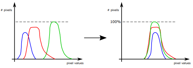
On a camera operation level, the white balance operation is performed previous to the debayering operation. The figure shows the gray levels distributions for the debayered image and for each of the three channels R, G, and B.
Before the white balance operation is correctly performed, the three different colors show different peaks. If your image has a histogram similar to the graph on the left it means that green will have higher values compared to the other two colors. So if you have a gray sample it will be shown with a color leaning toward green.
After the white balance has correctly been applied you will see the three graphs with the peak centered around the same value. When you reach this state you will see a gray having the same value in the three color channels.
The difference in the curves could happen due to the differences in the light spectrum and the sensor spectral quantum efficiency and are not preventing a correct white balance.
Anyway, by operating white balance in ITALA View you might also see that after the white balance operation the three curves are not only equalized on their mean gray levels, but also their distribution peak values are closer than before the white balancing. This happens because the white balance operation also adds a gain so that the 3 peaks are around the same value. However, as we discussed, white balance cannot control the curves’ distributions.
You can check the results of the White Balance by looking at the value stored under Balance Ratio Selector > Balance Ratio. The K factor of the selected color is saved in this variable.
You can use the same procedure also to set a different value and change manually the white balance of the image.
Color correction matrix
What it is
The Color Correction Matrix (CCM) is a mathematical matrix derived through color calibration processes that involve the characterization of the color properties of a specific imaging system. These matrices are often used to minimize color inaccuracies in an image and/or achieve accurate color reproduction according to specific color standards.
Why it is interesting
Achieving good color fidelity can be challenging because the color information of an image depends on the sensor’s color filter and the application’s illumination. The color correction matrix can be used to correct colorimetric errors, calibrate color reproduction, or match colors across different devices or lighting conditions.
By applying the color correction matrix, the colors in your image can be accurately transformed or corrected, ensuring consistent color appearance across different devices, color spaces, or lighting conditions in your machine vision applications.
This is particularly important for applications where color accuracy is crucial, such as color inspection, color sorting, or color analysis.
Machine vision softwares that take in consideration some types of color analysis must rely on an accurate color fidelity, which could have a great impact on the information extracted by the images and the application results.
How to set Color Correction Matrix
Color correction can be easily accomplished through the use of a reference color checker (such as a Macbeth chart seen below) and the Color Correction Wizard on ITALA View.
- Connect the camera and make sure that it is in free run acquisition.
- Select the Horizontal Line Profile tab and draw an ROI which includes only the grayscale values on the bottom of the color checker.
- Each greyscale tile of the displayed image should match the reference value imposed by the color checker. Therefore it’s necessary to adjust Exposure Time and Gamma values in order to achieve this perfect match. For now consider only the green channel.
- After this has been adjusted, use the Balance Ratio Selector and the Balance Ratio Feature to do the same operation also for Blue and Red Channels. When the Red, Green and Blue curves are superimposed, the white balance is optimal.
- Open the Color Correction Wizard (Wizard > Color Correction).
- Place the color checker in the Field of View, the Wizard guides you on the correct placement. Try to capture the whole color checker in the Field of View and make it fill as much frame as possible.
- Click and drag the 2 corners of the overlay matrix in order to center each overlay color target to the tiles of the color checker.
- Select X and Y ratio in order to consider only the center part of each color tile. Keep the overlay color targets distant from the tile's edges.
- Click the Correct button to start the color calibration.
- Wait until the end of the process.
- Click on Apply to save the changes.
- In order to make this change permanent, you should save the current user set. Loading the default user set will restore the factory color correction matrix.
Technical considerations
The Color Correction Matrix (CCM) operation allows to:
- achieve the best color fidelity related to the application needs by adjusting the output color components of the image.
- make conversions between color spaces, for example from RGB to YUV.
As for the White Balance (WB), in order to do the above operations the CCM algorithm defines the RGB pixel by a color vector whose three components are the gray levels of each channel R, G and B.
By doing this, we can describe the CCM operation as a mathematical calculation that converts the original color vector corresponding to a pixel, into a new color vector according to the following formula:
Rin, Gin and Bin values are the gray levels of each R, G and B component after the application of the white balance., while Rout, Gout and Bout values are the “corrected” gray levels of each R, G and B component in the image output by the camera.
The Gain and Offset coefficients can be freely edited by the user, or can be automatically calculated by following the instructions of the dedicated CCM wizard.
Both WB and CCM allow to improve the color fidelity of the image which is output by the camera to the host, so it is important to distinguish between these operations.
From the mathematical point of view, the WB algorithm targets the equalization of the three R, G, B components of the color vector, which condition is satisfied when:
The CCM allows the user to adjust the output values of the three color channels Rout, Gout and Bout and does not set any condition on their balancing. This allows the user more degrees of freedom in setting the correction coefficients for each color channel.
In the CCM algorithm the formula to calculate each output channel must take into consideration correction coefficients on all the three input channels. This means that in order to represent the Blue color correctly, you must take care also of the Red and Green colors input values. This makes the result more reliable and similar to what the human eye is able to achieve.
When applying the CCM the equations corresponding to each color channel is a function of all the inputs (i.e.: a linear combination):
On the other hand, the WB “correction matrix” could be represented as the CCM “correction matrix” where only the diagonal coefficients are preserved, and consequently each channel output Rout, Gout and Bout only depends on the corresponding channel input Rin, Gin and Bin. Then the white balance condition Gout=Bout=Rout introduces the relation between the three channels.
From the application perspective, the WB allows to compensate for illumination variability or intrinsic differences in light sensitivity at the sensor level. While this operation improves the color performances, the condition that the “white” color is balanced in the output image does not guarantee that each color component R, G and B is represented correctly by itself.
On the other hand, the CCM allows the user to precisely set the correction coefficients per each R, G, B channel. This operation can guarantee that each color represents exactly the information required by the application.
Real colors allow for example different types of Red, where the R channel is dominant with respect to the G and B channels, but where the proportion of each of the three channels is differently combined. What distinguishes two “real” Red colors is the different combination of all the three R, G and B components.
In this case the WB can not guarantee that two different types of Red colors are represented correctly in the output image, while the CCM can guarantee that.
In conclusion, despite both WB and CCM being able to improve the color fidelity in the output image, the WB purpose is not the color fidelity itself, its purpose is to maintain a balance between the three components of color in order to represent the "white" correctly. On the other hand, the CCM purpose is to allow the user to precisely set the desired R, G and B color components representation in the output image, and so CCM choice is recommended in order to achieve the best color fidelity according to the application needs.
The Color Correction Matrix is also used to make conversions between color spaces.
For example, if the user selects YUV pixel format for the output image, the camera automatically loads the right coefficients to switch from RGB to YUV color space.
This operation is performed automatically by the camera according to the standard conversion matrix which allows this color space transformation, and it does not influence the color fidelity in terms of compensating any possible color-biases introduced by the illumination or by the pixel sensitivity to different wavelengths.
For example, the correction matrix to convert from RGB to YUV color spaces is the following:
Note that CCM, as well as the debayering, is performed on-board to the camera only for RGB8 and YUV422 pixel formats. Images captured with raw pixel formats (BayerRG / BayerGR / BayerBG / BayerGB) are output to the host without debayering and CCM operations. Both the debayering and the CCM must be performed by the software when Raw Pixel Formats are selected.
CCM is usually performed also by monitors in order to give you a visual feedback of the acquired image that is as similar as possible to the colors seen by your eyes.