Optimizing system resolution: a practical guide to matching lens and sensor MTF

The purpose of this document is to guide you in the best possible choice regarding the correct matching between the camera and optics. We will see how to match the MTF of the camera with the one of the optic and we will dive deep into the concept of resolution in a machine vision application.

If you are looking for technical details on the products, their features and specifications, we recommend that you always refer to the product manuals.

Resolution is a fundamental concept in optical imaging and the broader field of machine vision. However, the term can be ambiguous as it refers to two distinct concepts. The first, and more straightforward, definition is the sensor's total pixel count (e.g., 5 megapixels). The second, more nuanced definition, concerns spatial resolution: the size of the smallest detail a system can distinguish within the captured image. This technical note will focus on the latter, providing a theoretical framework for calculating the achievable spatial resolution of a vision system using specifications from camera and lens datasheets. 

The primary tool for this analysis is the Modulation Transfer Function (MTF) chart, which encapsulates the essential performance data of an optical system. Properly matching a camera and lens is paramount, especially in applications where the defects to be detected are minuscule relative to the overall Field of View (FOV). As a rule, the size of the smallest feature you need to identify dictates the target resolution for your system. 

For any image processing software to perform a reliable analysis, a feature must not only be resolved but also rendered with sufficient contrast across multiple pixels. Critically, as a fundamental guideline derived from the Nyquist-Shannon sampling theorem, the smallest feature of interest must span at least two pixels to be reliably sampled and digitally represented. 

In machine vision, image quality is not defined by aesthetic or emotional criteria, as it is in photography. Instead, a "good" image is one where the contrast is optimized for a specific task, which typically involves one of two goals:

• Resolving features of interest with enough clarity for software to perform a correct analysis.

• Suppressing irrelevant details that might otherwise interfere with the analysis.

Ultimately, the primary goal of a machine vision system is to generate optimal contrast for the application. The resolution of the lens and sensor determines the system's ability to capture the smallest required features with sufficient contrast. The Modulation Transfer Function (MTF) is the key metric used to quantify this capability.

Conceptually, a system's transfer function describes its ability to transfer spatial information from the object (the input) to the image (the output) without loss. The MTF specifically measures the system's response to patterns of varying spatial frequencies, typically expressed in line pairs per millimeter (lp/mm). An MTF chart plots the percentage of contrast retained on the y-axis against the spatial frequency on the x-axis. For instance, if a sinusoidal pattern with 100% contrast at a given frequency is presented to the system, the MTF value indicates the percentage of contrast that will be present in the final image. This analysis assumes that any object can be represented as a sum of these sinusoidal frequencies (a principle of Fourier analysis).

It is crucial to note that spatial frequencies in the object space are scaled to the image space by the system's magnification. For a more in-depth definition of MTF, please refer to our Basics section.

The true power of the MTF lies in its application within the frequency domain. This allows for a straightforward, modular analysis of a complete vision system. The MTFs of individual components, such as the lens and the sensor, can be simply multiplied together to determine the total system MTF. This is significantly simpler than the equivalent operation in the spatial domain, which would require a more complex mathematical convolution. This powerful principle enables engineers to predict the final system's performance by combining the specifications of its constituent parts, ensuring the lens and camera are appropriately matched to achieve the desired resolution and contrast.

The performance of a machine vision system stems from the synergy among its components: lighting, optics, camera sensor, electronics, digitization, and software. This paper highlights how the integration of optics and sensors contributes to system performance, with a focus on optimizing their match to achieve the required resolution.

This chapter focuses on how to evaluate this critical pairing by analyzing their respective Modulation Transfer Functions (MTFs).

While the complex mathematical derivation of these curves is beyond the scope of this document, the essential behavior to understand is universal: both lens and sensor MTFs invariably decrease as spatial frequency increases. This downward trend signifies a fundamental trade-off: the finer the detail an application requires, the lower the contrast the system will be able to resolve.

It is crucial to recognize that every component in the imaging chain contributes to this overall loss of contrast; the final system performance is a product of these individual limitations. The following sections will, therefore, delve into the specific factors that shape the MTFs of lenses and sensors. Understanding these individual characteristics is the first step toward intelligently combining them to create an optimized and effective vision system.

The resolution of any lens is not infinite; it is constrained by two primary factors: the physical laws of diffraction and the practical imperfections of optical aberrations.

1. The Diffraction Limit: The Physical Boundary

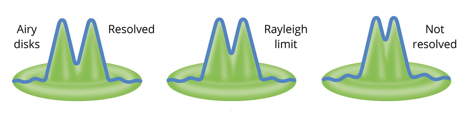
Diffraction is a fundamental phenomenon dictated by the wave nature of light. Even a perfect, aberration-free lens cannot focus light from a point source to an infinitesimally small point. As light passes through the lens's circular aperture, it diffracts and spreads out, creating a pattern known as the Airy pattern. This pattern consists of a bright central spot, the Airy Disk, surrounded by concentric rings of diminishing intensity.

The size of this Airy Disk represents the smallest possible spot a lens can create, thus setting its ultimate theoretical resolution limit. The radius of the Airy Disk is defined as the distance from its center to the first minimum of the pattern:

where:

• λ is the wavelength of light.

• f/# is the f-number of the lens (focal length / aperture diameter).

According to the Rayleigh criterion, two adjacent point sources are considered distinguishable, or "resolved," when the distance between the center of the Airy Disks is larger than their radius. This establishes the theoretical best-case resolution for any optical system.

2. Optical Aberrations: The Practical Limitation

While diffraction sets the theoretical best-case scenario, aberrations represent the practical imperfections inherent in any real-world lens design. They arise from the lens's geometry, material properties, and manufacturing tolerances, preventing light rays from converging to a single perfect point. There are many types of aberrations, including spherical, chromatic, coma, and astigmatism.

Calculating the combined effect of these aberrations is a complex task, typically performed using specialized optical design software. Their impact is what separates the performance of a real lens from that of a theoretically perfect, diffraction-limited one. For a more detailed explanation of specific aberrations, please see our Basics section.

Visualizing Performance on the MTF Chart

The MTF chart provides a comprehensive visual representation of how both diffraction and aberrations impact a lens's performance.

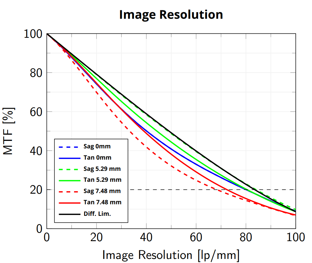
On a typical lens MTF chart, you will find:

• The Diffraction Limit (Black Colored Line): This curve represents the theoretical maximum performance of a perfect lens, limited only by the physics of diffraction at a given f-number and wavelength.

• Actual MTF Curves (Colored Lines): These show the real-world performance of the lens at different points within the image field (e.g., center, mid-field, corner). The gap between the diffraction limit and these curves quantifies the performance loss due to optical aberrations.

• Tangential (Solid) and Sagittal (Dashed) Lines: For each field position, two curves are often shown (e.g., a solid and a dashed line of the same color). These represent performance in two perpendicular orientations (tangential and sagittal). A separation between them indicates the presence of off-axis aberrations like astigmatism and coma.

The Critical F-Number (f/#) Trade-Off

One of the most important adjustments that directly impacts the MTF is the lens's f-number. Varying the aperture creates a critical trade-off between diffraction and aberrations:

• Low f-numbers: This setting improves the diffraction limit (the Airy Disk is smaller). However, a wider aperture allows light rays to pass through the lens at steeper angles, which significantly increases the effect of most optical aberrations. In this state, the system is typically aberration-limited.

• High f-numbers: This "stops down" the lens, reducing aberrations because the light rays passing through are more central and parallel to the optical axis. However, the smaller aperture increases the effects of diffraction (the Airy Disk becomes larger), lowering the theoretical performance limit. In this state, the system becomes diffraction-limited.

Finding the optimal f-number is a balance between these two competing factors.

Lens Cut-Off Frequency

Finally, the spatial frequency at which the lens contrast drops to zero is known as the cut-off frequency. Above this frequency, the lens cannot resolve any detail. It is determined by the diffraction limit and is calculated as:

Just like a lens, an image sensor has its own Modulation Transfer Function (MTF) that characterizes its ability to resolve detail. While a sensor's resolution is fundamentally linked to its pixel size, other factors also significantly influence its MTF. These include the sensor's architecture (e.g., front-side vs. back-side illumination), the pixel's fill factor, and the presence of microlenses over each pixel. The sensor MTF is a critical metric, as it allows for a direct, quantitative comparison between the performance of the sensor and that of the lens.

When analyzing a sensor's MTF, two key frequencies are of particular importance: the sensor cut-off frequency and the Nyquist frequency.

1. Sensor Cut-off Frequency: The Physical Pixel Limit

A sensor is composed of a discrete array of pixels. By definition, any detail smaller than a single pixel cannot be individually represented in the captured image. This physical limitation dictates that the sensor's transfer function must eventually fall to zero. The spatial frequency at which this occurs is known as the sensor cut-off frequency, and it corresponds to a detail size equal to one pixel pitch. It can be calculated as:

At this frequency, and for all frequencies above it, the sensor's contrast response is zero.

2. The Nyquist Frequency: The Practical Sampling Limit

While the cut-off frequency defines the absolute physical limit, a more critical boundary for practical system design is the Nyquist frequency. When a continuous optical image is projected onto the sensor, it is "sampled" by the discrete grid of pixels. This digitization process is governed by the Nyquist-Shannon sampling theorem.

The theorem states that to accurately reconstruct a signal, the sampling rate must be at least twice the highest frequency present in that signal. In imaging terms, this means that the smallest feature you wish to resolve reliably must be sampled by at least two pixels. If this condition is not met, a phenomenon known as aliasing may occur, where high-frequency details are incorrectly represented as lower-frequency patterns, creating artifacts like moiré patterns that corrupt the image data.

The Nyquist frequency defines this critical threshold and is exactly half of the sensor's sampling frequency (which is the inverse of the pixel pitch). It is calculated as:

Designing for Success: Staying Below the Nyquist Limit

Any spatial frequency in the image that falls between half of the Nyquist frequency and the sensor cut-off frequency is in a "danger zone" where aliasing is likely to occur. Therefore, when designing a machine vision system, the sensor must be chosen such that the highest spatial frequency required by the application remains below the half of sensor's Nyquist frequency. This ensures that all features of interest are sampled correctly, leading to accurate and reliable image analysis.

We have established that both the lens and the sensor have their own MTF curves that describe their individual performance. The power of the MTF methodology lies in how easily these can be combined. Because the analysis operates in the frequency domain, the total MTF of the paired system is calculated by simply multiplying the MTF of the lens by the MTF of the sensor.

This calculation provides a robust prediction of the final image contrast the system can deliver at any given spatial frequency.

To visualize this, consider a system using a Telecentric lens (e.g., TC23056) and a camera with a 3.45 µm pixel size. The graph below plots the MTF of each component individually, alongside the resulting System MTF.

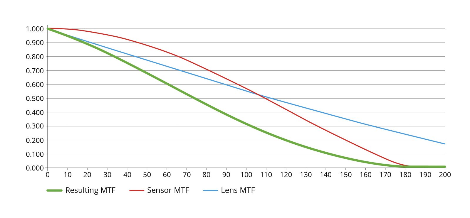
The MTF graph shows on the x-axis the spatial frequency expressed in line pairs over millimeters and on the y-axis the contrast.

Contextualizing the MTF: Other Critical System Factors

While the System MTF is a powerful predictor of optical and sensing performance, it is one piece of a larger puzzle. To apply this knowledge effectively in a real-world application, we must also be mindful of other contributing factors:

• Illumination and Object Contrast: The MTF describes how well a system transfers existing contrast, but it is the lighting strategy that generates the initial contrast on the object. The performance predicted by an MTF analysis, which often assumes ideal high-contrast conditions (like a backlight), can change significantly based on the chosen illumination.

• Image Digitization: The camera's bit depth and pixel format dictate how the analog contrast captured by the sensor is converted into a digital value. A system with excellent optical contrast may still fail if the bit depth is too low to resolve the necessary grayscale information.

• Software's Interpretive Capability: Ultimately, the image analysis software must be able to work with the resulting digital image. The threshold for "sufficient contrast" is not absolute; it is defined by the software's algorithms and the specific task at hand.

A common initial approach to pairing a lens and sensor is to match the radius of the lens's Airy disk to the sensor's pixel size. The logic is that if the smallest spot of light from the lens covers a 2x2 pixel area, the Nyquist criterion is satisfied.

However, this "Airy disk rule" is overly simplistic and can be misleading for several reasons:

• It ignores aberrations: In most real-world scenarios, especially at wider apertures (low f-numbers), optical aberrations, not diffraction, are the dominant factor limiting a lens's resolution.

• It misrepresents the f-number trade-off: The rule implies that lower f-numbers (which produce a smaller Airy disk) are always better. In reality, the best lens performance is often found at mid-range f-numbers where there is an optimal balance between aberrations and diffraction.

• It is based on point sources: The Airy disk describes the image of a single point of light. Machine vision applications analyze complex surfaces characterized by a wide spectrum of spatial frequencies, which are more accurately described by the MTF.

For these reasons, a far more robust method is to analyze the interaction between the complete MTF curves of both the lens and the sensor.

Analyzing the Lens-Sensor Interaction: Three Common Scenarios

When we plot the lens MTF (blue), the sensor MTF (red), and the resulting System MTF (green), three distinct scenarios typically emerge.

Case 1: The Optics-Limited System

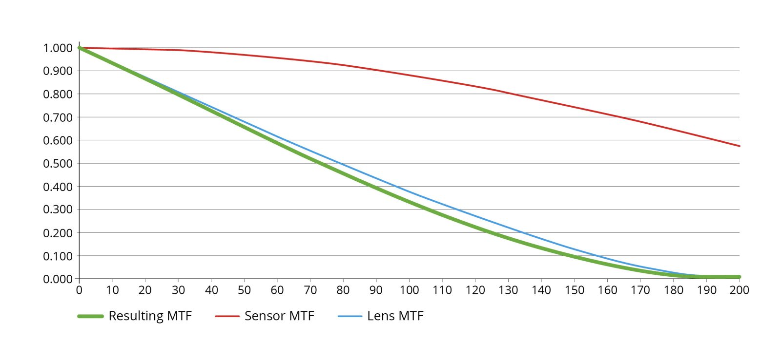
In this case, the lens MTF drops off significantly faster than the sensor MTF. The lens is the clear bottleneck, and the sensor's higher resolution capability is underutilized. The sensor is effectively oversampling the blurry image produced by the lens.

Case 2: The Sensor-Limited System

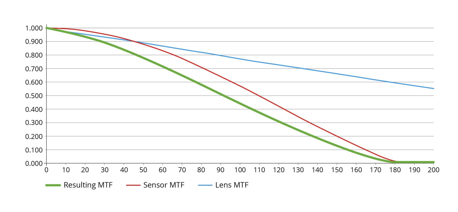
Here, the lens is capable of resolving very fine details with high contrast, but the sensor's Nyquist frequency cuts off the system's performance prematurely. The lens's high-resolution potential is wasted because the sensor is undersampling the sharp image. This is often the least desirable scenario, as it carries a high risk of aliasing artifacts.

Case 3: The Balanced System

This scenario represents a well-matched pairing. The lens performance degrades gracefully and intersects the sensor's Nyquist frequency at a meaningful contrast level. Both components contribute to the final system performance without one severely overpowering the other.

Design Trade-offs and Optimization

While a balanced system is often the ideal starting point, the other scenarios can be strategically acceptable depending on application constraints:

• If your system is Optics-Limited: You have an opportunity for optimization. Since the lens is the bottleneck, you could potentially switch to a sensor with larger pixels (and thus lower resolution). This would not significantly degrade the final image quality but could offer other benefits like higher frame rates, better light sensitivity (SNR), or lower cost.

• If your system is Sensor-Limited: You are likely paying for lens performance that you cannot use. You could select a less powerful (and likely cheaper or more compact) lens without a noticeable drop in the final image quality, reducing system cost and complexity.

A Quantitative Guideline for a Balanced System

While visually inspecting the MTF curves is insightful, a quantitative rule of thumb is useful for design. A guideline for achieving a well-balanced system is that:

The lens MTF should have 30% contrast at 67% of the Nyquist Cutoff Frequency.

This simple check provides a robust, data-driven starting point for selecting a lens and camera that are well-matched for your application's specific resolution needs.

So far, our analysis of MTF has focused on performance in the image space that is, on the sensor itself. However, the features we need to resolve exist in the object space. To bridge this gap and make practical component choices, we must incorporate optical magnification into our calculations. This chapter outlines a systematic process for selecting the right lens and camera based on your application's specific needs.

Step 1: Define the Required Object Resolution

The starting point for any system design which requires resolution performance is to define the minimum feature size that must be resolved on the object. This is the single most important parameter and could be:

• The smallest defect you need to detect.

• The finest detail you need to measure.

• The smallest object you need to identify.

Let's call this value the Smallest_Feature_Size, expressed in micrometers (µm).

Step 2: Convert Object Resolution to Image-Side Spatial Frequency

Next, we must translate this requirement from the object space into the spatial frequency that the lens and sensor system will need to resolve in the image space. This frequency, expressed in line pairs per millimeter (lp/mm), depends directly on the system's magnification. The formula is:

Note: A "line pair" consists of one dark line and one bright line. Therefore, to resolve a feature of a given size, we need to resolve a pattern with a period of twice that size, which explains the factor of 2 in the denominator.

Step 3: Define the Minimum Required Contrast

Once an image is captured, analysis software must be able to reliably distinguish the features of interest. If the contrast at the required spatial frequency is too low or zero, that information is effectively lost, and the software will fail.

While some algorithms can work with very low contrast, a robust and reliable system requires a safety margin. Based on extensive field experience, a common "rule of thumb" is to target a minimum contrast of 20% at your required spatial frequency.

Why 20%? This conservative threshold accounts for several real-world factors that will inevitably degrade contrast further and are not included in a simple MTF calculation:

• Imperfect Illumination: The MTF model assumes a perfect 100% contrast on the object, which is rarely achievable with real-world lighting.

• Additional System Components: The true system MTF is a product of all components, including optical filters, camera electronics, and digitization processes, each adding a small amount of degradation.

• Real-World Features: The model assumes perfectly sinusoidal patterns, whereas real defects and features have complex shapes.

• Noise: All electronic systems have inherent noise (from the sensor, lighting, or electronics) that reduces the signal-to-noise ratio and makes low-contrast features harder to detect.

Therefore, targeting a 20% contrast from your lens-sensor combination provides the necessary headroom to be reasonably confident that your application works reliably under real-world conditions.

Putting It All Together

With these three steps, the design process becomes clear:

1. Identify the smallest feature you need to see.
2. Calculate the required spatial frequency based on your chosen magnification.
3. Choose a camera which image sensor satisfies the Nyquist criterion
4. Choose a lens which best matches the sensor resolution
5. Confirm that the combined System MTF curve shows a contrast value of at least 20% at the application’s required spatial frequency.

This data-driven approach transforms component selection from a trial-and-error process into a more reliable procedure.

Having covered the theoretical framework, let's apply it to a real-world scenario. This case study will walk through the process of selecting and verifying a camera and lens combination for a specific application.

1. Defining the Application Requirements

First, we establish the core parameters for our inspection task:

• Required Object Resolution: We need to resolve features as small as 45 µm.

• Required Field of View (FOV): The inspection area is 54 mm × 45 mm.

2. Selecting a Suitable Sensor

Our first step is to determine the minimum sensor resolution needed. According to the Nyquist-Shannon sampling theorem, we need at least two pixels to resolve our smallest feature. Therefore, our effective sampling size in the object space must be half of the target resolution:

We can now calculate the minimum number of pixels required for our sensor:

• Horizontal Pixels: 54,000 µm (FOV) / 22.5 µm = 2400 pixels

• Vertical Pixels: 45,000 µm (FOV) / 22.5 µm = 2000 pixels

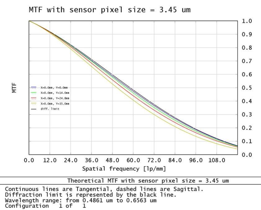
A sensor with a resolution of 2400 × 2000 pixels (or 4.8 megapixels) would meet this requirement. A standard 5-megapixel industrial camera, such as the ITA50-GM-10C, is an excellent candidate. This camera features a sensor with a 3.45 µm pixel size.

3. Selecting a Suitable Lens

With a sensor chosen, we can now select a lens. The primary parameter is magnification, calculated as:

This must be calculated in both the x and y directions, and the lowest magnification must be considered. In this case, using the specifications of the ITA50-GM-10C camera, the resulting magnification is 0.157x

We need a lens that meets three criteria:

1. Magnification: Should be lower than 0,157x, as close as possible to the exact value of 0.157x (for a fixed-magnification lens).
2. Image Circle: Must be larger than the sensor's diagonal (11 mm for the ITA50-GM-10C).
3. Mount: Must be compatible with the camera (e.g., C-mount).

The TC23056 telecentric lens is a perfect match, offering a magnification of 0.157x, an 11 mm image circle, and a C-mount.

4. Verifying the System Performance with MTF Analysis

We have selected our components. Now, we must verify that their combined performance meets our goals using the MTF methodology.

Step 4a: Calculate the Required Spatial Frequency

First, we convert our 45 µm object resolution requirement into the corresponding spatial frequency on the image sensor using the formula from the previous chapter:

This is our target frequency. Our system must deliver sufficient contrast at 71 lp/mm.

Step 4b: Check for a Balanced System

Before calculating the final system MTF, we can quickly check if the lens and sensor are well-matched. The sensor's Nyquist frequency is:

First, it is necessary to verify that the sensor’s Nyquist frequency remains at least twice the required spatial frequency as the introduction of lens magnification may has affected the condition previously satisfied by the sensor resolution alone. In this case this is true.

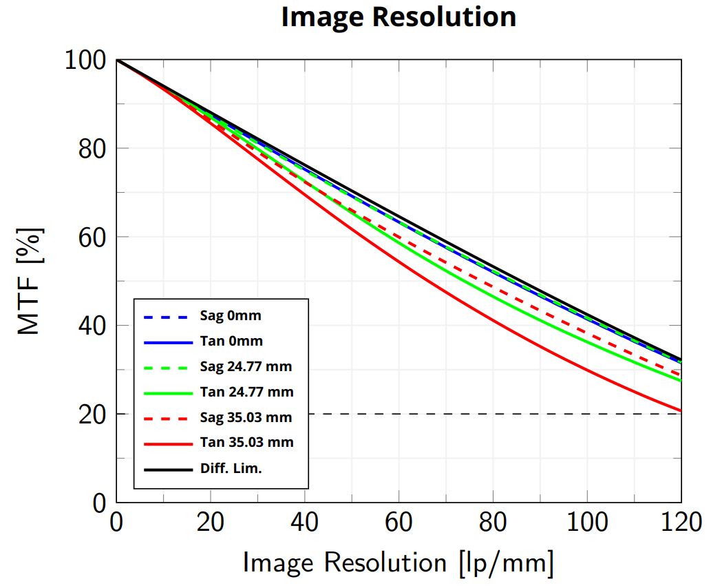
To properly match the lens and camera resolutions, we should now consider if the lens MTF can achieve 30% contrast at 67% Nyquist Cutoff Frequency, which corresponds to about 97 [LP/mm].

Looking at the MTF chart for the TC23056 lens, we find that its contrast at 97 [LP/mm] is between 30% and 40% in all the field of view.

Step 4c: Analyze the Final System MTF

We now multiply the lens and sensor MTFs to get the final System MTF curve.

By examining the System MTF graph, we can confirm our most critical requirement:

• At our target frequency of 71 lp/mm, the system delivers a contrast of over 30% across the entire field of view.

This comfortably exceeds our 20% minimum contrast rule of thumb, confirming that the chosen system is robust and well-suited for the application.

5. Determining the System's True Resolution Limit

As a final step, we can use the MTF graph to determine the absolute resolution limit of our lens and camera system. By finding the spatial frequency where the system MTF curve drops to our 20% contrast threshold (approximately 86 lp/mm), we can calculate the smallest feature the system can reliably resolve:

Smallest Resolvable Feature = 1000 / (2 ⋅ 86 lp/mm ⋅ 0.157) ≈ 37 µm

Conclusion of the Case Study

Our analysis confirms that the combination of the ITA50-GM-10C camera and the TC23056 lens is an excellent choice. The system not only meets the initial requirement of resolving 45 µm features but is capable of reliably resolving details as small as 37 µm, providing a healthy performance margin for this application.

Throughout this technical note, we have journeyed from the fundamental principles of resolution to a practical, data-driven methodology for choosing and matching lens and camera based on the needed application resolution. We have demonstrated how to:

• Evaluate the performance of individual lenses and sensors using their Modulation Transfer Function (MTF).

• Understand how critical parameters like a lens's f-number and a sensor's pixel size shape their respective MTF curves.

• Predict the performance of a complete system by multiplying the component MTFs and analyzing whether the system is optics-limited, sensor-limited, or well-balanced.

• Apply a systematic, quantitative approach to match a lens and sensor to specific application requirements.

The central takeaway is this: achieving optimal resolution is not a matter of simply choosing the component with the highest specifications. Instead, it is a process of intelligent system design, where the lens and sensor are carefully selected to work in synergy.

The process should always begin with the application's needs: a clear definition of the smallest feature that must be resolved within a given Field of View. These two parameters are the bedrock of the entire design. From there, the MTF provides a powerful framework to translate these requirements into concrete component choices, moving beyond guesswork and toward predictable, reliable results.

By adopting this MTF-based methodology, you are equipped to build vision systems that are not just functional, but truly optimized for clarity, precision, and performance. This data-driven approach is the key to unlocking the full potential of your machine vision applications.